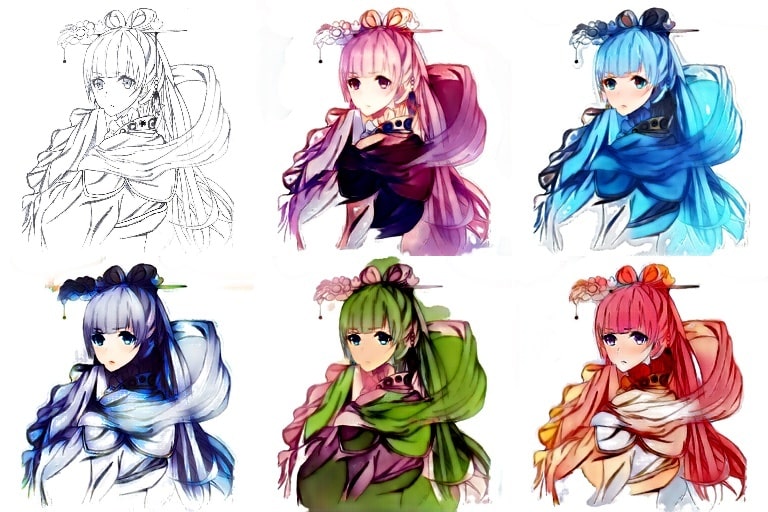
Five different outputs from the colorization model. Source lineart image (top left) was drawn by my friend @kuronaken.

Introduction

Recently I stumbled across Kevin Frans’ DeepColor project, which uses pix2pix (Isola et al. 2017) to colorize lineart images, given the original greyscale lineart image and a “color hint”, which is a rough guideline of which colors go where. This automates the coloring process, which comprises a significant portion of the time and effort taken when creating digital art. Nifty!

Results from DeepColor. Left: Lineart + “color hint”. Right: Generated image (source)

However, pix2pix needs to be trained with paired examples to work well. In many cases, paired data may be difficult or impossible to obtain (e.g. zebras ↔ horses). In DeepColor, lineart + color image pairs are used. The color images are scraped from Safebooru, and the corresponding black & wite lineart images are created by thresholding color images which results in the grainy artifacts seen above. The pix2pix generator manages to filter these out and there are ways to reduce the amount of artifacts (I found median blurring to work the best), but this denoising process causes the model to ignore fine features like noses and mouths (see above again). Ideally we would be able to train the model with real lineart images to best represent the distribution of input lineart images.

In comes CycleGAN!

To address the limitations mentioned above, the authors of pix2pix created CycleGAN (Zhu et al. 2017), which applies the cycle consistency loss to GANs, aiming to “capture the intuition that if we translate from one domain to the other and back again we should arrive at where we started”.

Let’s say we have an image of a horse and an image of a zebra. Our horse2zebra generator G is trying to transform the horse, x, into an image G(x) that (hopefully) looks like a zebra. The cycle consistency loss says that if we run that transformed image G(x) through the zebra2horse generator F, we should now end up with an image F(G(x)) that looks like the original horse x that we started with. So basically we want F to be the inverse function of G, effectively making F(G) an identity function.

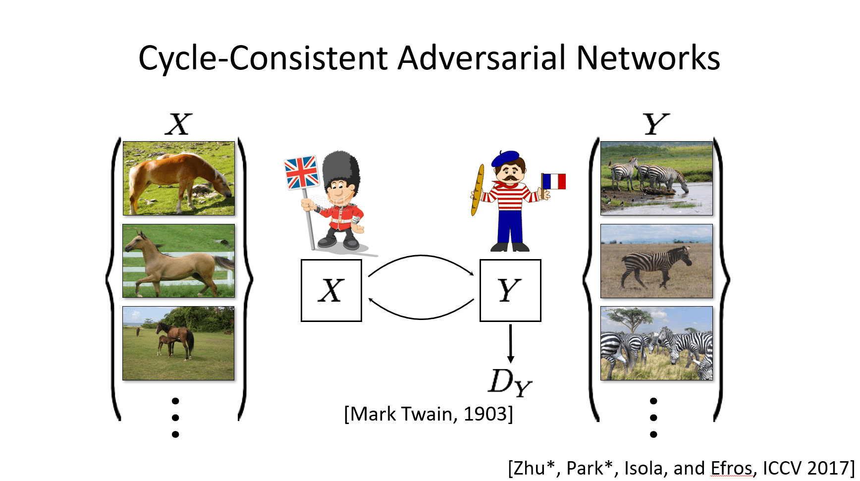Illustration of cycle consistency, from the ICCV 2017 presentation. (source)

Although CycleGAN was published in 2017 (which by deep learning standards is quite old), cycle consistency is still a crucial component of unpaired image-to-image translation methods at the time of this writing, as seen in U-GAT-IT (Kim et al. 2020), which to my knowledge is currently SOTA.

CycleGANime

To better understand how CycleGAN works, I implemented it myself with the same goal of colorizing lineart images. Using the authors’ PyTorch implementation as a reference, I wrote a minimal implementation of CycleGAN. Scripts are also included to concurrently download images from Safebooru.

Results

The best results are shown at the beginning of this post. The network manages to color within the lines quite nicely. It also learned some important things, like coloring the hair a different color than the face. Some results even manage to have unique eye colors.

Let’s take a closer look at one of the rows:

Results for one lineart image. Top left is the input image A, and the rest are results from different training iterations.

The model manages to preserve fine details, and there’s not much noise in the output either. It even learns to use multiple colors, for example coloring the hair a different color than the clothes. Neato!

The results don’t always look this nice though. The output of the model heavily depends on the images from the latest batch, even when learning rates approach zero. Here’s an example of one of the bad batches.

Bad results. I actually don’t watch anime often, so I have no idea who any of these characters are :\

The best method I found to get good results was to compute results and save their corresponding models often, then pick the best one at the end. With a dataset of ~2000 un-paired images (1000 lineart, 1000 color), it took about 50 epochs to start getting decent results, so after that point I began saving results + weights every 100 iterations or so.

Deployment

Since CPU inference only takes a few seconds, I deployed the model on a GCP e2-medium instance (free credits yay!). The frontend site was built with Vue and the backend is a Flask+Gunicorn microservice, using Redis as a task queue.

What didn’t work

I had a few other ideas on trying to squeeze out the best results from the network that didn’t work:

Training the network on the (few) test images

I tried limiting the training set to the images used for visualization (test set) because I thought that it would make the model better. My intuition was that the model would only have to learn the mapping from a few lineart images to the full set of color images, allowing it to specialize in just the few images that it was trained on. Instead, the model became delusional and created some pretty crazy looking results.

What happens when you only train on a few input trainA lineart images- even with the full set of trainB images, the model quickly becomes delusional. Most of these delusional results looked like nightmare fuel, so instead here I’m showing one that looks cool.

Fine-tuning

Similar to the point above, when I trained on the full training set and subsequently tried to use a few test output color images to try and fine-tune the network to colorize in a specific style, the results quickly became saturated and degraded quickly.

GAN tricks

There are many failure modes one can encounter while training GANs and just as many proposals on how to remedy these as well as improve results. Some are included in the original implementation, but I tried a new new ones that didn’t work:

• Soft labels - Using 0.9 as the real label instead of 1: I didn’t notice any noticeable improvement, but it didn’t seem to hurt the model either.
• Manual loss balancing - Only updating the discriminator/generator when loss > x: I noticed that the results were noticeably worse when I used this method, even for a small x=0.05.

Conclusions

The cycle consistency loss enables image translation models to be trained without paired images, which allows us to colorize lineart without having to use noisy generated lineart images. While this method produces what I believe to be higher quality results, the user has less control over what the final product will look like. Nevertheless, I’m impressed by the model’s ability to color nicely and stay within the lines.

For future work, it would be interesting to see how newer methods like U-GAT-IT (Kim et al. 2019) work, and see how the many-to-many mapping (originally proposed by MUNIT (Huang et al. 2018) affects quality.

If you’re an artist and just want the best results possible, you’re better off using a tool like PaintsChainer or Style2Paints instead of this.

Credits

This project was inspired by Kevin Frans’ DeepColor project. Some of the lineart images used to test the model were drawn by my talented friend (@kuronaken). Images were scraped from Safebooru. Code is based off the CycleGAN authors’ PyTorch implementation.

Appendix: Technical details

Here I’ll list some implementation details that I think are worth mentioning:

• I found that increasing the generator capacity had a greater improvement on the quality of results than the datasets used in the original paper, which I think is because coloring and shading lineart in an artistic manner is a more difficult task than just changing the color and texture of an object (e.g. apple↔orange or horse↔zebra). While the 6 block model struggled to color nicely and stay within the lines, the 9 block model had better shading, and the 12 block model started to learn to paint in different colors, and even coloring in eyes. Tested on 256x256 images.
• Normalizing the input lineart images helps improves the consistency of the results. I’m not talking about just rescaling the pixel values between -1 and 1 or subtracting pixel means, but iteratively brightening/darkening the non-white pixels until the average pixel intensity reaches a certain value. Without this, some images may have white patches while others have black patches in the same batch. This value also affects the results too: too bright, and the results look washed out. Too dark and results are too dark. Interestingly the model doesn’t learn to fix this itself. I found an average pixel intensity of around 180-200 to work the best.
• The L1 identity loss in the implementation requires that A and B be the same shape. I tried getting rid of it because I wanted to input 1 channel instead of 3 channel grayscale images to the model (just feels more true to the task, ya know), but the results had a clear lack of structure, so I had to revert it.